Scientific Machine Learning to simplify hydrological modelling in a changing climate

Keywords

vadose zone, modelling

What has been done with Scientific Machine Learning in hydrology and related fields so far?

Over the past few years SciML has been explored in different hydrological studies. Karpatne et al. (2017) introduced the need for a solution like SciML with an example from hydrological modelling from Ghasemizade and Schirmer (2013). Subsurface flow mechanisms are still insufficiently understood, due to lack of direct measurements at field and catchment scale, and due to non-linear interactions between complex non-linear sub-processes. Therefore, mechanistic hydrological models often have poor performance and have limited physical interpretability, because they often have many parameters that are difficult to interpret. Pure data-driven approaches however lack the properties to help better understand natural systems. SciML might therefore prove a path forward to overcome these shortcomings.

In a hydrological SciML study, Jia et al. (2020) combined process-based modelling with machine learning to predict river water flow and river temperature. They did this for both observed and unobserved river segments, which are connected to eachother and therefore affect eachother. Different, but connected, river segments can have different water flow and thermodynamic behaviour due to differences in catchment characteristics and drivers.

Often, few river segments are actually observed. Availability of measured data is thus limited in river hydrology. Process-based models in hydrology are approximations of the environment that suffer from omission of processes due to incomplete knowledge or to limit computational costs. Although these models contain general physical relationships expressed in mathematical formulae, they also contain parameterisations based on qualitative properties of the catchment, like soil and land cover. (Jia et al. 2020)

Due to the interaction between different river segments and data scarcity, making a successful representation of a river by building a separate machine learning model for each separate river segment (e.g. setting up a Recurent Neural Network; RNN), is impossible (Jia et al. 2020). To build a successful representation, Jia et al. (2020) combined the RNN-approach with the Graph Convolutional Neural Network (GCN) approach. The latter technique captures both spatial interactions and temporal dynamics. GCN methods however, do not contain physical knowledge about the interactions between different neural network nodes. When learning is done with sparse and less representative data, a GCN model can become non-generalisable. Jia et al. (2020) therefore used intermediate variables from a process-based model to guide the GCN learning process (hybrid physics-ML modelling). Individual segments are trained first, with synthetic data. Then, the complete (i.e. global) ML model is trained with a loss function that takes care of consistency with local patterns.

Another SciML-study in hydrology was carried out by Bhasme, Vagadiya, and Bhatia (2021). They used the term physics informed machine learning and predicted streamflow while using machine learning to estimate evapotranspiration as an intermediate variable and streamflow as a final output variable. Estimating intermediate variables with machine learning are an approach that falls within the category of physics-guided machine learning architecture design.

Two separate machine learning models were embedded in the structure, with the estimation of actual evapotranspiration being a function of precipitation, soil moisture content at the previous time step, and potential evapotranspiration (Bhasme, Vagadiya, and Bhatia 2021). The streamflow was a function of the precipitation, soil moisture content at the previous and the same time step, groundwater storage amount at the current and previous time step, and actual evapotranspiration. This model was compared to a machine learning model with precipitation and temperature as inputs and streamflow as output, and with the original physics-based model. Within both the pure machine learning approach and the SciML approach, different learning algorithms were tested. The comparison was done for ten different catchments in India. This SciML approach yielded good, and in some cases better, water balance estimates compared to purely physics-based modelling and compared to pure machine learning. In other words, the SciML-approach has the ability to outperform the more traditional methods. This study also showed that SciML can help make rigid physics-based hydrological models more flexible.

In a research field closely related to hydrology, crop science, Maestrini et al. (2022) reviewed the state of both mechanistic and data-driven crop modelling. Furthermore, he explored the possibilities of combining the best of both approaches for yield prediction. Choices made by mechanistic crop model developers on the level of detail of different processes, are simplifications that lead to biases in model outcomes (Maestrini et al. 2022). On the other hand, data-driven approaches do not use domain knowledge, their results can not be extrapolated, and they need large datasets to be trained, especially if patterns are non-linear and if complex interactions occur. Therefore, also in crop science there is a need for the SciML-approach.

The literature review of Maestrini et al. (2022) on crop modelling showed that data-driven approaches were more often used at larger spatial scale (e.g. county and larger) and physics-based modelling was used more often at field and farm scale. This might not be surprising, because at smaller scale more detailed (management) data, which is needed for input, calibration, and validation of physics-based models, is usually available due to intensive monitoring at specific sites. However, machine learning was also used to predict yield at field scale. Even, a deep learning neural network approach, which needs a large amount of data, was used with maize breeders’ trial data. It outperformed other techniques including shallow neural networks and regression tree, among others. Such approaches are becoming more feasible, because the amount of (publicly) available remotely sensed (e.g. satellite and drone) and near-sensing (e.g. agricultural vehicle-based) data has increased and have allowed for an increase in machine learning popularity for yield prediction. Still, a major bottleneck for machine learning in crop modelling, is that large amounts of different types of data are still limited in availability. This is to a certain part due to different ownership of different datasets and privacy issues related to this.

Maestrini et al. (2022) set out three main cases for integrating data-driven and mechanistic approaches in crop modelling:

1. use mechanistic models to develop new indices and to expand the predictor space of data-driven models
2. use data-driven models to produce unavailable mechanistic model inputs like soil properties
3. metamodels, mainly to reduce computational cost

Maestrini et al. (2022) found a few (successful) applications in crop science of both incorporating physics-based modelling in data-driven models (1) and the other way around (2).

More concretely, Maestrini et al. (2022) proposed a new methodology based on metamodeling and transfer learning. Transfer learning is a technique in which a number of layers of a neural network is trained on a certain task and then, after training extra layers and possibly retraining the layers trained already, using the neural network to execute another task. A simple and popular example is to train a neural network to recognise images of cats and then use it to recognise images of dogs. The model input must be of the same form for both tasks, so both must be images in the case of the cats and dogs images example. The more similar the two tasks are, the beter this technique performs. More distant tasks have a greater chance of leading to worse performance of a transferred model than of a model trained on target data only. Such result is called ‘negative transfer’. An example of using transfer learning in agricultural research is a study by Suh et al. (2018), which transferred a neural network for image classification to classification of sugar beet leaf health status.

Maestrini et al. (2022) see a need for crop growth metamodels employing neural networks trained on synthetic datasets, which are then transferred to the target task, using a smaller, more specific dataset. They thereby want to bring knowledge from mechanistic models into data-driven models. A major challenge to the approach proposed, is the lack of large, standardised data sets of field scale observational data.

Machine Learning and Scientific Machine Learning in Vadose Zone Hydrology

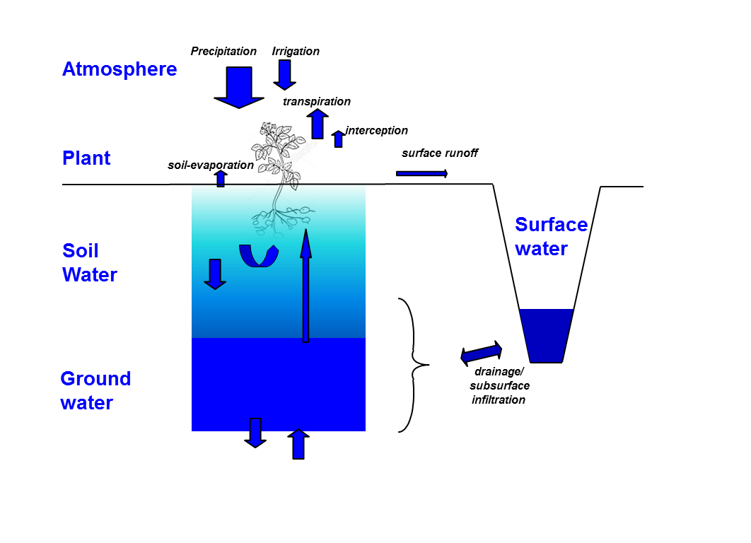
In literature a commonly used word for the unsaturated, or better said, the variably saturated part of the soil, is the vadose zone. On this website we use this term.

The movement of water in the vadose zone is often modelled with the Richardson-Richards’ equation (“Weather Prediction by Numerical Process” 1922; Richards 1931). This equation is based on the Buckingham-Darcy equation and assumes conservation of mass, an incompressable porous medium (which is not always acceptable in clay soils and peat soils) and a constant liquid density (acceptable in most cases in agriculture and other environments). Solving the the Richardson-Richards’ equation (numerically) is non-trivial and computationally expensive.

Recently Ghanbarian and Pachepsky (2022) shared a communication on the use of machine learning in vadose zone hydrology. They mentioned that hydrologists and soil scientists were early adopters of machine learning techniques. The application has been mostly regarding pedotransfer functions. Pedotransfer functions are formulas that translate soil properties like soil composition information (e.g. sand, silt, clay, and organic matter contents) to soil hydraulic properties, like hydraulic conductivity and water retention capacity. A well-known example is the Rosetta model (Schaap, Leij, and van Genuchten 2001; Zhang and Schaap 2017), which was constructed using an artificial neural network.

Another application of machine learning targeted relatively often in modelling the vadose zone, is the construction of metamodels. Metamodels, both based on machine learning and other techniques, have been applied in vadose zone hydrology to limit the high computational costs of running physics based soil hydrologcal models when applied at for instance regional scale. An example of a metamodel that includes the vadose zone to an important extend, and that uses machine learning is part of ‘WaterVision Agriculture’ (Hack-ten Broeke et al. 2016). It is based on the vadose zone model SWAP (Dam et al. 2008) and the plant physiological model WOFOST (Boogaard et al. 1998).

WaterVision Agriculture

SWAP

WaterVision Agriculture was developed to calculate the effects of hydrological measures on annual average agricultural production in the Netherlands. This model allows to compute effects under both the current climate and future climate. It can do so while distinguishing between effects on agricultural production from drought, too wet conditions (oxygen stress), and salinity in the root zone. Besides different climate scenarios, the metamodel takes as input 72 different soil units typical of The Netherlands, multiple crop types, and groundwater dynamics. Groundwater dynamics input is provided as a yearly average largest and a yearly average smallest groundwater table depth, which the user can set with a precision of 1 cm. The model then searches a database to find the closest model run available within it. This database was build with a random forest (Breiman 2001) of regression trees. A random forest is a machine learning technique that employs the decision tree technique, using IF-ELSE statements.

More recently, beyond common machine learning, SciML has been explored in vadose zone hydrology (Ghorbani, Sadeghi, and Jones 2021; Bandai and Ghezzehei 2021; Tartakovsky et al. 2020). Especially, the PINN method (Maziar Raissi, Perdikaris, and Karniadakis 2017a; Maziar Raissi, Perdikaris, and Karniadakis 2017b) has been investigated. However, different techniques have been used as well. In the next sections we provide an overview of what has been done on this matter.

PINN-approach in vadose zone hydrology

Tartakovsky et al. (2020) applied the physics-informed deep learning (PINN) method established by Maziar Raissi, Perdikaris, and Karniadakis (2017a) and Maziar Raissi, Perdikaris, and Karniadakis (2017b) to approximate partial differential equations and the pedotranfer functions used within them. They estimated saturated and unsaturated hydraulic conductivity and hydraulic pressure. They used measurements of saturated hydraulic conductivity and hydraulic head for saturated flow and capillary pressure head for unsaturated flow. The partial differential equations used were Darcy for saturated flow and Richardson-Richards’ for unsaturated flow. These PDEs were constrained by minimising the PDE-error at selected points. The PINN-method yielded more accurate approximations of partial differential equation estimates than traditional deep learning. Saturated hydraulic conductivity was estimated with higher accuracy when the PINN-method was used, compared to more traditional approaches. The relationship between hydraulic pressure and conductivity was estimated accurately with the PINN-method when employing only (noisy) matric pressure measurements.

While soil hydrological parameter values from laboratory experiments are available, these can not simply be transferred to field scale, at which soil hydrological modelling usually takes place. More accurate parameter value estimates at field scale can however be estimated with inverse modelling, using field scale observations. Bandai and Ghezzehei (2021) applied the PINN-method to estimating soil water retention curves, hydraulic conductivity functions, and to solving the Richardson-Richards’ equation. One advantage of using the PINN-approach in this case was that no explicit boundary or initial conditions are needed. Another advantage was that no good prior estimations of the soil hydraulic functions are needed. Yet another advantage was that the shapes of the soil hydraulic functions do not need to be defined beforehand. Using only synthetic soil volumetric water content data from HYDRUS1D simulations (Šimnek et al. 2008) with synthetic noise added, they obtained functions that could simulate the true volumetric water content dynamics. Both the soil water retention curves and hydraulic conductivity functions were simulated accurately by the PINNs at mid-range soil water content, in nonparametric form. At the dry and wet ends however, both soil hydraulic functions were not estimated well, due to non-linearity not captured by the neural networks. The PINNs simulated soil water flow well with noisy synthetic soil moisture flow data.

Despite the limitations shown by the outcomes, the fact that the PINN-method can provide useful nonparametric soil hydraulic functions with only volumetric soil content and no initial or boundary conditions, is interesting at least. There are multiple ways forward from this finding. First of all, the approach has been limited to synthetic data and homogeneous soil profiles. Applying it to vertically heterogeneous soils and using real observations is considerably more complicated. To cater for heterogeneity, monotonicity needs to be build in according to Bandai and Ghezzehei (2021), as elaborated on by Daniels and Velikova (2010). Another limitation is that the PINN implementation of Bandai and Ghezzehei (2021) cannot handle well sharp gradients and strong non-linearity. Bandai and Ghezzehei (2021) propose the residual-based refinement method from Lu et al. (2019) to meet this challenge. Another issue is the optimisation of the neural network architecture (number of hidden layers and number of nodes). Within this study, the soil water flux was used for this purpose, but this variable is not usually observed in the real world. As a solution to this, Bandai and Ghezzehei (2021) proposed to use the training error, which is defined in terms of the volumetric water content, to optimise the architecture (Mishra and Molinaro 2020). So, to use the PINN-approach in field-scale soil hydrology in practice, further work needs to be done.

Bandai and Ghezzehei (2021) built further on the work of Tartakovsky et al. (2020), by using (synthetic) volumetric water content data instead of (synthetic) soil matric potential (i.e. soil hydraulic pressure) data. The advantage of using volumetric water content is that such data is more readily available. That is despite that soil water pressure observations should actually be the preferred option, if available. Soil water flow is directly related to differences in spatial soil hydraulic head. Physical knowledge is added to the neural network approach through the PINN loss function, which contains two separate terms for both the comparison with observational data and for the comparison with the physics-based differential equation(M. Raissi, Perdikaris, and Karniadakis 2019). Moreover, Bandai and Ghezzehei (2021) successfully tested and applied the monotonicity constraint on both soil water retention functions. Monotonicity means that a function can yield increasing or decreasing values only, for increasing or decreasing input values. In other words, the derivative does not change sign (plus versus minus). This constraint makes physical sense because, soil hydraulic conductivity and soil hydraulic head (which goes from strongly negative to small negative values) only increase (monotonically) with increasing soil water content. Technically, Bandai and Ghezzehei (2021) used three fully forward connected neural networks. One network was to estimate soil hydraulic pressure head from vertical space coordinates and time coordinates, thereby simulating the Richardson-Richards’ equation. The output of this network was then fed to both a neural network that yielded soil hydraulic conductivity and a neural network that yielded soil water content. Applying automatic differentiation, first and second order differentials were computed. These differentials are terms of the Richardson-Richards’ equation. The residual function of this equation is the physics-based loss term of the PINN loss function. On the neural network architecture side, another interesting detail is the choice of activation and output function types. The activation function of the first neural network part (with output hydraulic pressure) was chosen to be a hyperbolic because the Richardson-Richards’ function is a second-order partial differential equation. The matric potential (i.e. pressure head) must be negative and therefore a negative exponential was chosen as output function The tangent hyperbolic function was used as activation function of both soil hydraulic functions. Their output function of the soil water retention function was chosen to be a sigmoid, to assure output values between zero and one. The output function of the soil hydraulic conductivity function was an exponential function to obtain positive values.

Other SciML-approaches in vadose zone hydrology

Ghorbani, Sadeghi, and Jones (2021) took another step to develop scientific machine learning in vadose zone modelling. They developed a machine learning based second order partial differential equation, similar in shape to the Richardson-Richards’ equation. To do so, they assumed a fourth order partial differential equation and let the training of the machine learning algorithm determine which order terms were significant (i.e. non-zero) and which non-zero parameter values these got. The algorithm yielded an equation with only the first and second order derivaties, the same terms as the basic Richardson-Richards’ equation contains. Which terms come out as non-zero is interesting as such, because it is known that the first and second order derivatives relate to gravity-induced flow and moisture diffusion, and that for instance the fourth-order derivative relates to wetting from instability and gravitational fingering (Cueto-Felgueroso and Juanes 2009).

Employing the sparse regression method, Ghorbani, Sadeghi, and Jones (2021) solved an equation with observed soil moisture and modeled soil moisture time-derivatives. Thereby, coefficients for the different space-derivatives of the observed soil moisture were obtained. Like Bandai and Ghezzehei (2021), Ghorbani, Sadeghi, and Jones (2021) used synthetic soil moisture data and a homogeneous soil profile. To produce the synthetic data, they used actually observed near-surface soil moisture data as input for a HYDRUS1D-model. They used the HYDRUS1D output as a reference against the outcomes of the machine learning approach. THe HYDRUS1D soil moisture output was also used as synthetic training data for the machine learning algorithm.

The training showed that three to six years of soil moisture data was needed to obtain convergence on the soil hydraulic conductivity and soil water diffusivity parameters. However, when surface boundary conditions were replaced with sinusoidal functions, just a few weeks of data was needed for training. The original top boundary was taken from rather noisy surface flux measurements fed into HYDRUS1D. From comparing different scenarios with observations at different depths, Ghorbani, Sadeghi, and Jones (2021) found that high temporal variability in soil moisture (like near the soil surface) should be accompanied with a large spatial extent of the data. The method computes temporal and spatial derivatives and therefore sufficient observations in both space and time are needed. Vertical interpolation was found to successfully establish a partial differential equation.

Ghorbani, Sadeghi, and Jones (2021) propose to use more advanced differentiation techniques, like automatic differentiation. The approach of Ghorbani, Sadeghi, and Jones (2021) can be used to reduce the nonlinearity of vadose zone models. This can be achieved by establishing a physically consistent, linear or quasilinear partial differential equation that is able to describe spatiotemporal soil moisture variability accurately, under different boundary conditions.

Ghanbarian and Pachepsky (2022) argued that with a large expansion of machine learning use in vadose zone hydrology, there has been less attention to certain important aspects of applying this technique. Accuracy and uncertainty of machine learning are database-dependent, i.e. they differ between datasets to which the same machine learning technique is applied. Reproducibility is often insufficient, with data, models, and computer code often not publicly available (lack of delivery).

In disciplines including (vadose zone) hydrology and soil science, data are (spatial) scale-dependent. Therefore, applying a machine learning model built with data at a certain scale cannot simply be applied at another scale (Ghanbarian and Pachepsky 2022). Comparing different types of machine learning algorithms on the same problem is often not done, while this would help assess quality of study outcomes. Fundamental protocols for machine learning, including on data, are required for earth sciences, following examples like proposed for environmental sciences by Heil et al. (2021). Ghanbarian and Pachepsky (2022) conclude with a call to address fundamental questions about the application of machine learning in research. For instance, they mention the questions why machine learning models exist and if there is a limit to machine learning model accuracy and reliability and what that depends on.

Concluding, there is considerable space and need for SciML in vadose zone research. While the PINNs-method has been tested in a few cases (M. Raissi, Perdikaris, and Karniadakis 2019), we have not found a vadose zone study with the UDE-approach (Rackauckas et al. 2020). This might be due to the more recent development of this method, but also due to the complexity of solving the Richardson-Richards’ equation. While UDE-solutions for different partial differential equations are available online, we could not locate one for the Richardson-Richards’.

What is currently needed to advance scientific machine learning in (vadose zone) hydrology?

Our literature study on SciML in (vadose zone) hydrology shows the research so far has been limited, due to the novelty of the technique. Fundamental machine learning questions need to be addressed and different machine learning algorithms should be compared (Ghanbarian and Pachepsky 2022) Studies that employed SciML-approaches like PINNs, show there is work to be done, especially with regard to using real observations and heterogeneous soils. To our knowledge, no study has so far used the UDE-approach to solve the Richardson-Richards’ equation for vadose zone modelling. Due to the complexity of solving this formula numerically, this poses an interesting challenge to explore.

Besides solving the soil physics itself, the relation with other processes can be addressed by SciML. Upper (meteorology) and lower boundary conditions (groundwater level dynamics) could be approached with SciML-techniques. Complex and poorly understood soil features like macropores could be addressed with for instance hybrid modelling (replacing part of a physics-based model with a machine learning module). Developing SciML-based metamodels for vadose zone models like SWAP and HYDRUS1D could be interesting from the viewpoint of reducing computational costs.

Karniadakis et al. (2021) listed some challenges relevant to developing SciML for vadose zone hydrology:

• High-frequency patterns hard for PINNs to solve
• Learning multiphysics-systems simultaneously is computationally expensive. This cost could be reduced by learning the different processes separately first and then coupling the different networks.
• Neural Networks physics-informed loss-functions may fail in specific low-dimensional cases, like diffusion with irregular conductivity. This could be the case in hydrology and soil science.
• During training, different terms of the complex loss function of a physically-informed neural network compete and therefore convergence to the global minimum cannot be guaranteed.
• Lack of theoretical foundation of physics informed learning models.

So, it seems there are plenty of research opportunities.

When exploring a new topic, it makes sense to start easy. Willard et al. (2022) provided us with some direction from this perspective. Hybrid modelling is easiest to implement, whereas physics-guided loss functions and physics-guided architecture need more expertise. Given the complexity of the vadose zone and the Richardson-Richards’ equation, it seems easiest to start with model boundary conditions. Therefore, we started with a use case on replacing the Penman-Monteith evapotranspiration formula (an upper boundary condition to the Richardson-Richards’ equation). Further steps we intend to take are: to dive into solving the Richardson-Richards’ equation with SciML-techniques, to address macropore flow, to replace lower boundary conditions with SciML, and to build a metamodel for SWAP (Dam et al. 2008).

References

Bandai, Toshiyuki, and Teamrat A. Ghezzehei. 2021. “Physics-Informed Neural Networks with Monotonicity Constraints for Richardson-Richards Equation: Estimation of Constitutive Relationships and Soil Water Flux Density from Volumetric Water Content Measurements.” Water Resources Research 57 (2): e2020WR027642. https://doi.org/https://doi.org/10.1029/2020WR027642.

Bhasme, Pravin, Jenil Vagadiya, and Udit Bhatia. 2021. “Enhancing Predictive Skills in Physically-Consistent Way: Physics Informed Machine Learning for Hydrological Processes.” arXiv. https://doi.org/10.48550/ARXIV.2104.11009.

Boogaard, H. L., C. A. van Diepen, R. P. Rotter, J. M. C. A. Cabrera, and H. H. van Laar. 1998. WOFOST 7.1; User’s Guide for the WOFOST 7.1 Crop Growth Simulation Model and WOFOST Control Center 1.5. Technical Document / DLO Winand Staring Centre 52. SC-DLO.

Breiman, Leo. 2001. “Random Forests.” Machine Learning 45 (1): 5–32. https://doi.org/10.1023/A:1010933404324.

Cueto-Felgueroso, L., and R. Juanes. 2009. “A Phase Field Model of Unsaturated Flow.” Water Resources Research 45 (10). https://doi.org/https://doi.org/10.1029/2009WR007945.

Dam, Jos C. van, Piet Groenendijk, Rob F. A. Hendriks, and Joop G. Kroes. 2008. “Advances of Modeling Water Flow in Variably Saturated Soils with SWAP.” Vadose Zone Journal 7 (2): 640–53. https://doi.org/https://doi.org/10.2136/vzj2007.0060.

Daniels, Hennie, and Marina Velikova. 2010. “Monotone and Partially Monotone Neural Networks.” IEEE Transactions on Neural Networks 21 (6): 906–17. https://doi.org/10.1109/TNN.2010.2044803.

Ghanbarian, Behzad, and Yakov Pachepsky. 2022. “Machine Learning in Vadose Zone Hydrology: A Flashback.” Vadose Zone Journal 21 (4): e20212. https://doi.org/https://doi.org/10.1002/vzj2.20212.

Ghasemizade, Mehdi, and Mario Schirmer. 2013. “Subsurface Flow Contribution in the Hydrological Cycle: Lessons Learned and Challenges Ahead—a Review.” Environmental Earth Sciences 69 (2): 707–18. https://doi.org/10.1007/s12665-013-2329-8.

Ghorbani, Asghar, Morteza Sadeghi, and Scott B. Jones. 2021. “Towards New Soil Water Flow Equations Using Physics-Constrained Machine Learning.” Vadose Zone Journal 20 (4): e20136. https://doi.org/https://doi.org/10.1002/vzj2.20136.

Hack-ten Broeke, M. J. D., J. G. Kroes, R. P. Bartholomeus, J. C. van Dam, A. J. W. de Wit, I. Supit, D. J. J. Walvoort, P. J. T. van Bakel, and R. Ruijtenberg. 2016. “Quantification of the Impact of Hydrology on Agricultural Production as a Result of Too Dry, Too Wet or Too Saline Conditions.” SOIL 2 (3): 391–402. https://doi.org/10.5194/soil-2-391-2016.

Heil, Benjamin J., Michael M. Hoffman, Florian Markowetz, Su-In Lee, Casey S. Greene, and Stephanie C. Hicks. 2021. “Reproducibility Standards for Machine Learning in the Life Sciences.” Nature Methods 18 (10): 1132–35. https://doi.org/10.1038/s41592-021-01256-7.

Jia, Xiaowei, Jacob Zwart, Jeffrey Sadler, Alison Appling, Samantha Oliver, Steven Markstrom, Jared Willard, et al. 2020. “Physics-Guided Recurrent Graph Networks for Predicting Flow and Temperature in River Networks.” arXiv. https://doi.org/10.48550/ARXIV.2009.12575.

Karniadakis, George Em, Ioannis G. Kevrekidis, Lu Lu, Paris Perdikaris, Sifan Wang, and Liu Yang. 2021. “Physics-Informed Machine Learning.” Nature Reviews Physics 3 (6): 422–40. https://doi.org/10.1038/s42254-021-00314-5.

Karpatne, Anuj, Gowtham Atluri, James H. Faghmous, Michael Steinbach, Arindam Banerjee, Auroop Ganguly, Shashi Shekhar, Nagiza Samatova, and Vipin Kumar. 2017. “Theory-Guided Data Science: A New Paradigm for Scientific Discovery from Data.” IEEE Transactions on Knowledge and Data Engineering 29 (10): 2318–31. https://doi.org/10.1109/TKDE.2017.2720168.

Lu, Lu, Xuhui Meng, Zhiping Mao, and George E. Karniadakis. 2019. “DeepXDE: A Deep Learning Library for Solving Differential Equations.” CoRR abs/1907.04502. http://arxiv.org/abs/1907.04502.

Maestrini, Bernardo, Gordan Mimić, Pepijn A. J. van Oort, Keiji Jindo, Sanja Brdar, Ioannis N. Athanasiadis, and Frits K. van Evert. 2022. “Mixing Process-Based and Data-Driven Approaches in Yield Prediction.” European Journal of Agronomy 139: 126569. https://doi.org/https://doi.org/10.1016/j.eja.2022.126569.

Mishra, Siddhartha, and Roberto Molinaro. 2020. “Estimates on the Generalization Error of Physics Informed Neural Networks (PINNs) for Approximating a Class of Inverse Problems for PDEs.” arXiv. https://doi.org/10.48550/ARXIV.2007.01138.

Rackauckas, Christopher, Yingbo Ma, Julius Martensen, Collin Warner, Kirill Zubov, Rohit Supekar, Dominic Skinner, Ali Ramadhan, and Alan Edelman. 2020. “Universal Differential Equations for Scientific Machine Learning.” arXiv. https://doi.org/10.48550/ARXIV.2001.04385.

Raissi, Maziar, Paris Perdikaris, and George E. Karniadakis. 2017a. “Physics Informed Deep Learning (Part I): Data-Driven Solutions of Nonlinear Partial Differential Equations.” CoRR abs/1711.10561. http://arxiv.org/abs/1711.10561.

Raissi, Maziar, Paris Perdikaris, and George Em Karniadakis. 2017b. “Physics Informed Deep Learning (Part II): Data-Driven Discovery of Nonlinear Partial Differential Equations.” ArXiv abs/1711.10566.

Raissi, M., P. Perdikaris, and G. E. Karniadakis. 2019. “Physics-Informed Neural Networks: A Deep Learning Framework for Solving Forward and Inverse Problems Involving Nonlinear Partial Differential Equations.” Journal of Computational Physics 378: 686–707. https://doi.org/https://doi.org/10.1016/j.jcp.2018.10.045.

Richards, L. A. 1931. “CAPILLARY CONDUCTION OF LIQUIDS THROUGH POROUS MEDIUMS.” Physics 1 (5): 318–33. https://doi.org/10.1063/1.1745010.

Schaap, Marcel G., Feike J. Leij, and Martinus Th. van Genuchten. 2001. “Rosetta: A Computer Program for Estimating Soil Hydraulic Parameters with Hierarchical Pedotransfer Functions.” Journal of Hydrology 251 (3): 163–76. https://doi.org/https://doi.org/10.1016/S0022-1694(01)00466-8.

Šimnek, J, M Šejna, H Saito, M Sakai, and M Th Van Genuchten. 2008. “The HYDRUS-1D Software Package for Simulating the Movement of Water, Heat, and Multiple Solutes in Variably Saturated Media, Version 4.0.” HYDRUS Software Series 3: 315.

Suh, Hyun K., Joris IJsselmuiden, Jan Willem Hofstee, and Eldert J. van Henten. 2018. “Transfer Learning for the Classification of Sugar Beet and Volunteer Potato Under Field Conditions.” Biosystems Engineering 174: 50–65. https://doi.org/https://doi.org/10.1016/j.biosystemseng.2018.06.017.

Tartakovsky, A. M., C. Ortiz Marrero, Paris Perdikaris, G. D. Tartakovsky, and D. Barajas-Solano. 2020. “Physics-Informed Deep Neural Networks for Learning Parameters and Constitutive Relationships in Subsurface Flow Problems.” Water Resources Research 56 (5): e2019WR026731. https://doi.org/https://doi.org/10.1029/2019WR026731.

“Weather Prediction by Numerical Process.” 1922. Quarterly Journal of the Royal Meteorological Society 48 (203): 282–84. https://doi.org/https://doi.org/10.1002/qj.49704820311.

Willard, Jared, Xiaowei Jia, Shaoming Xu, Michael Steinbach, and Vipin Kumar. 2022. “Integrating Scientific Knowledge with Machine Learning for Engineering and Environmental Systems.” ACM Comput. Surv., January. https://doi.org/10.1145/3514228.

Zhang, Yonggen, and Marcel G. Schaap. 2017. “Weighted Recalibration of the Rosetta Pedotransfer Model with Improved Estimates of Hydraulic Parameter Distributions and Summary Statistics (Rosetta3).” Journal of Hydrology 547: 39–53. https://doi.org/https://doi.org/10.1016/j.jhydrol.2017.01.004.