Scientific Machine Learning
scientific models, machine learning, modelling
The best of two worlds
In research, a new modelling discipline is gaining a foothold. Different names are used to refer to this new methodology, but here we use the term Scientific Machine Learning, or short: SciML (Baker et al. 2019; Rackauckas et al. 2020). Other terms commonly used to refer to this novel work field, or sub-disciplines of it, are universal differential equations (Rackauckas et al. 2020), physically informed neural networks (Raissi et al. 2019), physics informed machine learning (Karniadakis et al. 2021), theory-guided data science (TGDS; Karpatne et al. (2017)), and physics-based deep learning (Thuerey et al. 2021). As the name ‘Scientific Machine Learning’ tells, it is a combination of two separate terms; machine learning and science, in which science refers to physically-based modelling. Traditionally, these two research domains have been worlds apart. However, over the recent years, methods have been developed that can combine both. Scientific Machine Learning integrates mechanistic (i.e. physics based) models and knowledge and machine learning techniques in a synergistic way (Willard et al. 2022; Karniadakis et al. 2021; Karpatne et al. 2017, 2019). Thereby, the idea is to get the best of two worlds.
On this page, we provide a summary literature review of SciML.
Physics-based modelling versus machine learning
In this chapter we introduce physics-based modelling and machine learning. We look at their differences and briefly on how they can be brought together to get the best of both worlds.
Physics-based modelling
In the environmental sciences and in environmental engineering, physics-based models are used to estimate the effects of natural phenomena and human interventions on the conditions in the environment. In hydrology, for instance, models estimate the effects on river discharge and groundwater levels. The outcomes are used to predict for instance floods and droughts. Physics-based models contain mathematical formula’s that are based on scientific knowledge and physical laws. To build these models, observational studies and experiments were carried out. Although these models are based on knowledge and include our understanding of nature, certain sub-processes and properties are understood less or are highly heterogeneous in space and time (Blöschl and Sivapalan 1995). In many cases, a lack of observations or the infeasibility to sample sufficiently at all (to address high spatio-temporal variability), cause the need for making assumptions and using empirical relations within physics-based models. Physics-based models therefore include empirical relationships to parameterise certain parts. In soil hydrological modelling, an example is the use of curves and their parameters that describe the pull-forces exerted by soil particles on water in between them. Physics-based models, like all models, although based on domain-knowledge, are thus inherently simplifications of nature.
Statistical Modelling and Machine Learning
A whole different type of modelling is statistical modelling. This traditional approach is empirical in nature and does not necessarily (explicitly) draw on process-knowledge. Correlations between different variables are explored and conclusions are drawn about these correlations’ strengths. Linear regression is a clear example of statistical modelling. Statistical modelling is, like mechanistic modelling, a long-standing discipline.
A newer, related discipline, that has been under increasingly rapid development over the past decade, is machine learning (Jordan and Mitchell 2015). Machine learning does not make direct use of domain knowledge within the model structure. It explores correlations between different variables and makes predictions on them. This technique is especially valuable when correlations between variables are highly non-linear and complex [reference]. There is no universally accepted definite difference between statistical modelling and machine learning. These two disciplines have different gravities, but overlap. A good starting point to read about machine learning is Wikipedia. Different explanations of the differences between statistical modelling and machine learning exist. Some sources describing it quite wel are Machine learning vs statistical modelling which one is right for your business problem, Bzdok et al. (2018), and Ley et al. (2022).
Physics-based modelling and machine learning
Both approaches mentioned above, physics-based modelling and machine learning, have their own strengths and limitations. Physics-based modelling has better extrapolation abilities and the results are interpretable because they can be directly related to changes in input parameters and input variables [reference]. Limitations of physics-based models are e.g. long computation times and limited transferability across spatial scales. Strengths of machine learning algorithms are short computation times (after initial training) and strong predictive power [reference]. Limitations are the limited interpretability of model structure and model outcomes, and limited extrapolation strength.
The limited interpretability has especially been a limitation for uptake of machine learning by the environmental sciences and engineering modelling community. For specific purposes however, machine learning has been used much by this community. Spatial statistics and parameter estimation are examples of disciplines that have long made use of machine learning algorithms. [reference]
Complete replacement of process-based models by machine learning models has however not been feasible. Domain knowledge and physics laws can not be completely replaced by machine learning. Moreover, in environmental sciences, observational data is often limited. This makes effective machine learning difficult because their results under these data-limited conditions are insufficiently robust and do not guarantee convergence (Raissi, Perdikaris, and George E. Karniadakis 2017). However, there need not be made a choice between either one of process-based models and machine leaning. That is where Scientific Machine learning comes into the equation.
Scientific Machine learning has been under development for some years now, with the first publications explicitly mentioning the discipline in 2017 (Raissi, Perdikaris, and George E. Karniadakis 2017). Before that time, attempts were made to incorporate physical knowledge in machine learning and vice versa. An example is pruning data-driven models on physical consistency, yielding model parameterisations that satisfy certain conditions after training (Karpatne et al. 2017). The new methods of SciML are however more advanced, providing a chance for further integration and development.
The driving force for the development of SciML is the limited success of data science methods in solving complex problems of natural sciences Karniadakis et al. (2021). A major cause of the mentioned limited success, is that results (e.g. a trained and validated neural network) are often not successfully extrapolated. Physical systems contain a large number of physical variables that are in many cases non-stationary in time and have complex interactions, resulting in limits on extrapolation of data-driven models. Another reason for lack of success of data-driven methods in the natural sciences, is that the goal often is to learn about natural processes, to understand cause-and-effect mechanisms. To that end, interpretable models (theories of system functioning) are needed. Traditional data-driven approaches lack interpretable mathematical formulas and so provide limited or no insight of a natural system under study. Using the best of both worlds, SciML involves the ability to learn models from large datasets and the knowledge accumulated by scientific discovery. This can be done by integrating knowledge in data-driven models to increase the chance of regression relationships found to represent causal relationships. Moreover, physically consistent models can be derived. SciML might even lead to a new definition of process understanding, if parts of mechanistic models are replaced by machine learning that yield effective extrapolatable models (Karniadakis et al. 2021).
Artificial intelligence, machine learning, and deep Learning
In this chapter we briefly introduce three different concepts that form the basis of scientific machine learning, from the machine learning side. We keep it brief and refer to publications, websites, and videos that provide good explanations on these methods.
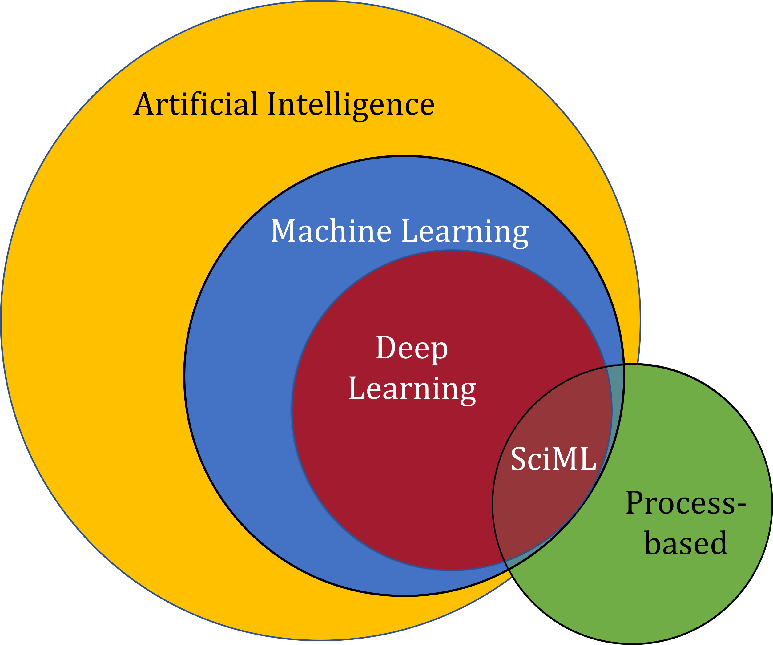
Artificial intelligence overarches machine learning. Machine Learning includes regression and classification techniques:
- Supervised and unsupervised (expand)
- Neural Networks (NNs) (expand)
- Representation learning (features are not hand -designed but learned by the algorithm) (expand)
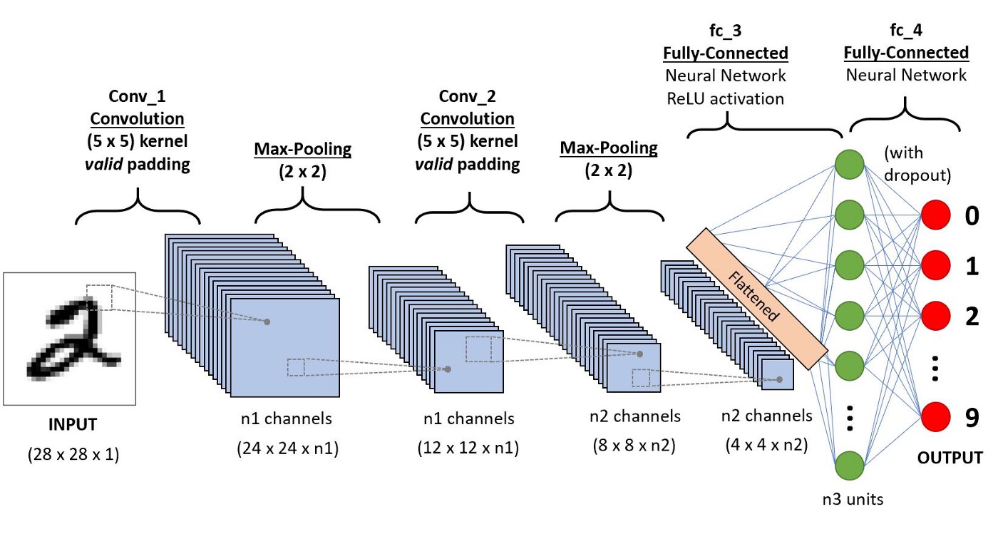
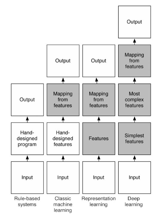
On its turn, machine learning overarches deep learning. Deep learning is thereby a sub-branch of machine learning (Goodfellow et al. 2016). There is no exact separation that states when a machine learning algorithm is deep learning or not. As seen in the comparing figure from Goodfellow et al. (2016) below, a deep learning algorithm extracts high-level abstract features (like the effect of day time on the colour of a car in an image or a person’s accent in a spoken language recording) by disentangling these into different simpler features. In an image this means that different simple features, like edges, combine to more complex features like object shapes. A deeper neural network allows to build complex features from simple features because the deeper layers accommodate combining the information from neurons in the higher layers.
In SciML, deep learning is often used, because it allows to separate complex pieces of information and use them to predict. As shown later, certain neurons or layers can be given (or reasoned to have) certain physical meanings.
Scientific Machine Learning (SciML)
Here we go deeper into the main SciML-topic. We provide an overview of what SciML is, which different SciML-techniques can be distinguished, and what has been done with SciML so far, in research domains related to soil hydrological modelling.
SciML objectives
Development of SciML can help address imperfections of mechanistic models, help to build more resource efficient mechanistic models, and can help to discover new knowledge (Willard et al. 2022). Different objectives to develop and use SciML from the perspective of improving computational techniques, stemming from the limitations of both process-based modelling and machine learning, were formulated by Willard et al. (2022). One is improving prediction performance, which means better matching between predictions and observations. Another is to improve sample efficiency, i.e. reducing the number of observations needed for adequate performance or to reduce solution search space. A third one is improving the interpretability of machine learning outcomes.
Introducing scientific knowledge can help to get a better understanding of processes. In environmental and engineering modelling, a range of objectives that help to improve modelling and process-understanding, i.e. from he application perspective, were formulated by Willard et al. (2022):
- to improve over physical models: combining physics-based models with ML-models;
- downscaling: Use machine learning to simulate at a finer resolution where that is needed for sufficiently good estimation of output variables. Especially dynamical downscaling (uses finer resolution simulations to estimate variables at a more local scale) is computationally expensive and can profit from machine learning techniques. Statistical downscaling (employs empirical methods to predict finer resolution variables from coarser resolution variables) can benefit from using neural networks, due to the complex and non-linear nature of cross-scale relationships.
- parameterisation: Parameterisation means replacing complex sub-processes with constants (i.e. static parameters). These parameters are usually calibrated. However, alternatively these sub-process representations can be replaced with machine learning models. This enables learning parameterisations directly from observations and modelling at high resolution.
- reduced-order models: “computationally less expensive representations of more complex models”. Machine Learning is starting to be used to aide construction of reduced-order models, to improve accuracy and to reduce computational costs. Applying physics principles could make more robust training of reduced-order models possible and could allow for successful training with less data.
- forward solving PDEs: Machine learning can be used instead of numerical solutions of partial differential equations. Computing numerical solutions (like the finite difference method) can be highly computationally expensive or even impossible in certain cases. On the other hand, machine learning based solvers often do not take physical laws into account. Recent developments however, like the construction of a solver for entire PDE families, employing a neural Fourier operator, provide a way forward.
- inverse modelling: Machine learning based surrogate models are becoming a realistic option for inverse modelling in environmental and engineering research, because they can cope with high dimensionality and because they are fast. Physics-based constraints are commonly used in traditional inverse problem solving. Incorporating such constraints in machine learning-based approaches can improve data-efficiency and help solve ill-posed problems.
- discovering governing equations: In research disciplines where dynamical systems have no formal analytical descriptions (e.g. neuroscience), despite abundant data, discovering governing equations with machine learning is an active field of research. Recent advances on this topic have been made with symbolic regression and sparse regression.
- data generation: Data generation approaches are used to synthetically simulate real scientific data. Traditionally, data generation was done with physics-based models or actual physical experiments. That is however time consuming and is restricted by what the chosen model can produce. Unsupervised machine learning provides a way forward that is less time consuming and that can provide more diverse data because there are no restrictions from the parameterisation chosen within a specific physics-based model.
- uncertainty quantification: To avoid the high computational expense of Monte Carlo modelling, deep learning-based surrogate models could be an interesting technique/ Integrating physics knowledge in such work can help better characterise uncertainty by, for instance, preventing physically inconsistent solutions, which in turn can reduce computational cost.
SciML-methods
To achieve the application-centric objectives mentioned in the previous section, different techniques can be used. Willard et al. (2022) listed four approaches:
- Physics-guided loss function: Standard machine learning methods can fail to capture complex relationships between physical variables at different scales, directly from data. This causes these models to not extrapolate well beyond their training space. Therefore, machine learning models consistent with physics are developed. One way to do this is by incorporating physical constraints in loss functions, by adding a term to them to penalise non-physical solutions (a weak constraint, i.e. it provides no guarantees non-physical solutions are completely excluded). This has, among other advantages, the advantage of improved out-of-sample generalisability. An example is the PINNs approach of Raissi, Perdikaris, and George Em Karniadakis (2017).
- Physics-guided initialisation: Physical knowledge can help to initialise (deep) neural network weights, to accelerate training and reduce the number of training samples needed. One technique used to this purpose is transfer learning (which employs pre-learning). Physics-guided initialisation can also be done with self-supervised learning (a method in-between supervised a unsupervised learning). In this method, deep neural networks are taught to differentiate between representations, using pseudo labels (labels made by applying a labelling model on unlabeled data). To our opinion, this can be useful in environmental and hydrological modelling because certain sub-processes (intermediate variables) can be predicted, to then pre-train machine learning models.
- Physics-guided design of architecture: Making black-box architectures more interpretable. Neural Networks, compared to other machine learning methods are especially useful to adaptations that incorporate physical knowledge into their architecture. For instance, specific neurons and connections between neurons can be given physical meaning. Another example is to base the choice of activation function on knowledge of the physical processes (Karpatne et al. 2017). One use of this technique is that physically meaningful information can be extracted from a neural network. The approach of adding physics-based information to neural network architecture is also used in solving differential equations
- Hybrid physics-ML models: Hybrid physics-ML models contain two models in one: a physics-based model and a machine learning model connected to it. An easily understood example is to replace part of a physics-based model with an ML-module. Another example is residual modelling, which involves training/calibrating a model, to improve its predictions. See also Karpatne et al. (2017).
Using SciML-methods
The overview of methods provided gives a chance to orientate on possible ways to apply SciML. However, Willard et al. (2022) also provided insight on what is needed for implementation of the techniques mentioned, what they can yield, and what is easier to start with and what is harder. The requirements and possible benefits per method were listed as:
- Physics-guided loss function
- Requirement: known physical relationship (e.g. PDE)
- Possible benefits: physical consistency, improved generalisation, reduced observations required, improved accuracy
- Physics-guided initialisation
- Requirement: Synthetic data from mechanistic model for training
- Possible benefits: Reduced observation required, improved accuracy
- Physics-guided design of architecture
- Requirement: Intermediate physical variables/processes, or hard constraints, or task interrelationships, or informed prior distributions
- Possible benefits: Interpretability, physical consistency, improved generalisation, reduced solution search space, improved accuracy
- Hybrid physics-ML models
- Requirement: operational mechanistic model during run time
- Possible benefits: improved accuracy
Willard et al. (2022) mentioned hybrid modelling as most simple to implement. The physics-guided loss function approach requires domain knowledge, to determine what to add to the loss function. Physics-guided architecture is a more complex approach and requires both domain knowledge and machine learning expertise. The different techniques can be combined in one modelling exercise.
Two well-known SciML-techniques
Physics-informed neural networks (PINNs)
An already relatively often used technique is physics-informed neural networks [PINNs; Raissi, Perdikaris, and George E. Karniadakis (2017); Raissi, Perdikaris, and George Em Karniadakis (2017); Raissi et al. (2019)]. A PINN solves a supervised learning task under the condition of respecting physics laws described by nonlinear partial differential equations. Two methods can be used with PINNs (Raissi, Perdikaris, and George E. Karniadakis 2017): (1) solving partial differential equations (given certain fixed model parameter values, what can be said about the unknown, hidden system state; a forward problem) and (2) discovering partial differential equations (i.e. finding the model parameter values that describe observed data best, so an inverse problem).
A difference between the PINN-method and earlier works that combined physics-based models with machine learning, is that previous methods used machine learning in a back-box way. By developing tailor-made activation functions and loss-functions for the differential operators, an understanding of the structure of the machine learning parts can be obtained.
An important technique that is used within this framework is automatic differentiation. Automatic differentiation is a family of differentiation techniques that uses the basic structure of computational algorithms, which consists of sequences of arithmetic operations, to obtain derivatives. The chain rule is used repeatedly to obtain the derivatives. Automatic differentiation is fast, employ efficient code, has no round-off errors, and can effectively compute higher-order derivatives.
According to Raissi et al. (2019), PINNs can be trained wih relatively little data, which is often the situation in real-world environmental modelling problems. The underlying reason for this property is that solutions that do not fit the physics-based equations are penalised in the loss-function. The PINN namely has a residual term from the mathematical equation of the physics-based model in the loss function [cuomo-etal-2022]. The PINN-method thus employs the physics-guided loss function method listed by Willard et al. (2022).
One challenge of continuous time PINNs, is that a large number of collocated points is needed to enforce physics-based constraints in the entire spatio-temporal domain. This plays a role in higher-dimensional problems because the number of points needed increases exponentially with increasing dimensionality. Techniques like quasi Monte-Carlo sampling and Runge-Kutta time-stepping can help here, to build discrete time models.

Mariodeff, CC BY-SA 4.0, via Wikimedia Commons
Universal differential equations for SciML
Rackauckas et al. (2020) introduced Universal Differential Equations (UDE) for SciML. A UDE is a differential equation with universal approximators incorporated. Rackauckas et al. (2020) built and provided a modular computer code based toolkit for the UDE-approach. The toolkit allows to solve a wide range of differential equation based scientific problems. An informative starting point is Scientific Machine Learning by Chris Rackauckas.
According to Rackauckas et al. (2020), the advantage of their approach over the PINN-approach is that they incorporate numerical techniques from physics-based modelling that have yielded stable, efficient solvers. For stiff models (models that need a small time step even when the response curve/surface is very smooth) the PINN-approach is computationally intensive. Even with some approaches like the before-mentioned discrete-model PINNs that partly overcome this challenge, a limitation still is that PINN-software does not allow to automatically combine the training process with efficient solving techniques available.